Quote:
Using stv014's MLS tone generator for the signal, GoldWave to record, HOLMImpulse to manipulate the recording/impulse response, a helper program I made to apply HRTF compensation to frequency responses exported to/from HOLM, and the command line version of Convolver (on SourceForge) for the convolving.
I am not sure if anyone finds this useful, but I have an updated utility package available:
dsputils.zip (last updated: 03/31/13). This still includes the old "mls.exe" program, but also several new ones, and the source code (those who use Linux can compile them with a command like "
g++ -Wall -O2 -ffast-math convolve.cpp -o convolve -lsndfile -lm -s" for each program, or simply "
make" to compile all; you can also add more optimization flags, and -DUSE_SIMD=1 for a very limited use of SSE2. If -DUSE_OOURA_FFT=1 is added to the compiler flags, then Takuya Ooura's
FFT library will be used, which is more efficient than the default FFT code, and is recommended. -DNO_FFT_TABLES=1 disables the use of tables in the Ooura FFT library; this reduces the memory usage slightly, but is not as fast, and normally not very useful. The code works correctly when compiled for 64-bit systems).
The programs included are:
convolve.exe - convolves a sound file with another, or one of several built-in filters. The input file is automatically resampled if the sample rate does not match that of the impulse response, and a sample rate adjustment factor can also be applied to correct the DAC/ADC clock frequency mismatch when extracting an impulse response from a recorded MLS. It supports multichannel files, and different number of channels in the input and IR file:
- N channel input, 1 channel IR: all channels of the input are convolved with the mono IR, output will have N channels
- N channel input, N channel IR: each channel of the input is convolved with the corresponding channel of the IR, output will have N channels
- 1 channel input, N channel IR: the mono input is convolved with each channel of the IR, writing N channels of output
- N channel input, N*N channel IR: any channel of the input can be convolved into any of the N output channels, the IR contains channel combinations in the order C1->C1, C1->C2, ..., C1->CN, C2->C1, ..., C2->CN, and so on. This can be used for crossfeed effects, for example
The built-in filters are MLS (it can be reversed for IR extraction, or upsampled for DAC filter measurements), lowpass, highpass, bandpass, notch, and comb bandpass and notch. All of the latter actually use some simple windowed waveform as the impulse response, and the user can set the length and type of the window. The impulse response can be processed to create inverse, minimum phase, and linear phase filters. Finally, it is possible to apply a gain both overall and separately for each output channel.
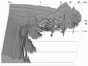
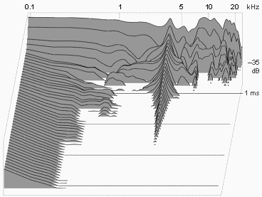
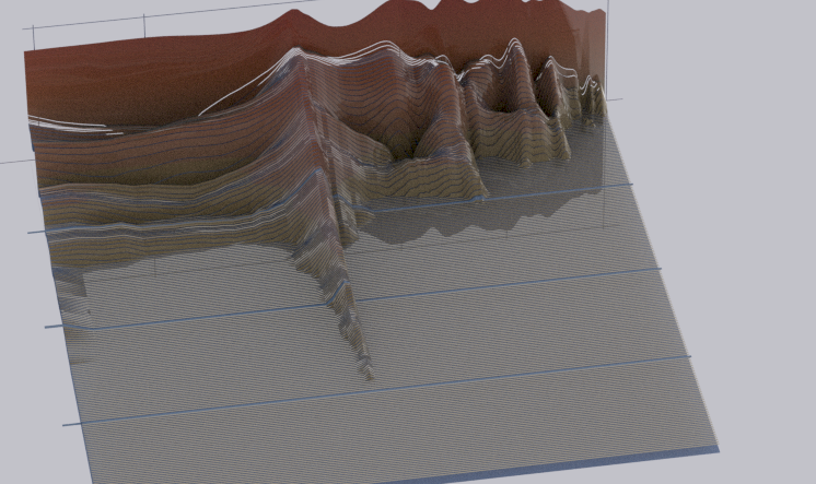
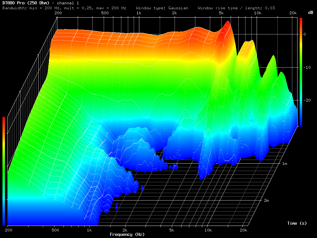
csd.exe - creates a CSD graph from an impulse response, and saves it as a 1024x768 256-color BMP file. See also
this post for an explanation of the analysis parameters.
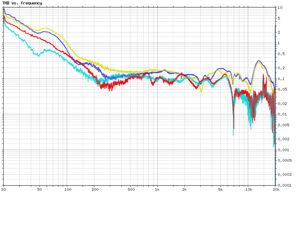
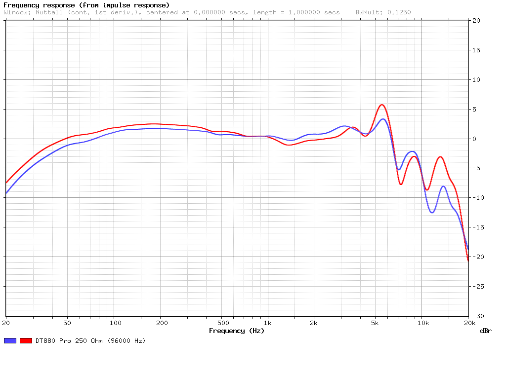
 fft.exe
 - creates an FFT plot from one or more audio file(s), and saves it as a BMP file, similarly to
csd.exe. It can be used in any of the following modes:
- "ir" (this is the default): magnitude response (dBr or raw) from impulse response
- "tone": similar to above, but the graph is scaled such that a 0 dBFS sine wave will be displayed as 0 dB, rather than a 0 dBFS impulse
- "freq", "thdf": frequency response or THD (dBr or %) vs. frequency from the output of
thd_test
- "lvl", "thdl": linearity (level error) or THD vs. level (raw, dBr, or Vrms) from the output of
thd_test
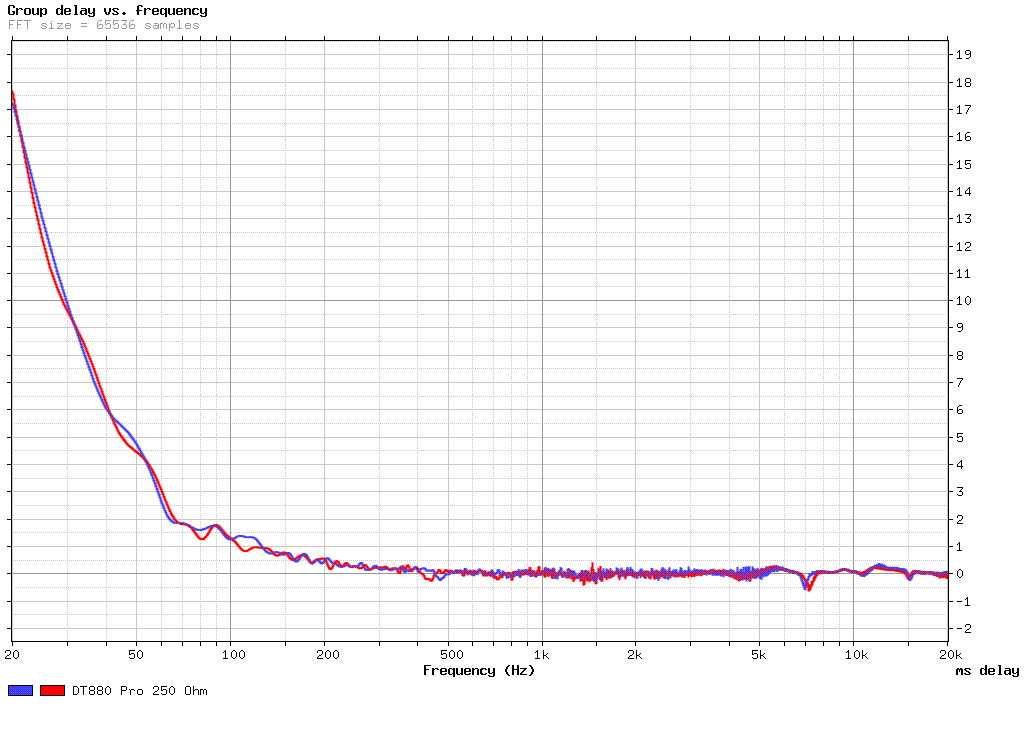
- "phs", "pd", "gd": phase (degrees), phase delay (ms), or group delay (ms) from the output of
groupdel
- "imp", "iphs": impedance magnitude (Ω) or phase (degrees) vs. frequency from the output of
impedance
Some features:
- up to 7 stereo input files can be displayed on a single graph (it would look rather cluttered, though)
- the color of each trace can be set to one of 14 colors:

- multichannel input files are supported, and will use more than one stereo slot (so, you can display 3 4-channel files and a stereo one, for example)
- more than 10 window types are supported, with any length up to 16777216 samples
- linear or logarithmic scale (both X and Y) with adjustable range
- optional smoothing (this is not supported in "phs", "pd", "gd", and "iphs" mode, and is mainly recommended for "ir")
- the title of the graph, and the description of each file can be changed, and the analysis parameters (window type, etc.) are printed


 groupdel.exe
 - analyzes the phase response, phase delay, or group delay of an impulse response. It does not actually display the results, but writes another WAV file, which contains an impulse response for FFT analysis in an audio editor (that is, 1 dB on the "frequency response" will mean 1 ms of group delay or phase delay, or 10 degrees of phase). By default, the output is calibrated for correct FFT display using
fft.exe, or in Cool Edit Pro with a 65536 sample Blackmann-Harris window; if the 0 dB level is wrong in other software, it can be adjusted with a command line parameter. The program that is used for FFT display needs to be able to read float samples without clipping, and preferably support an FFT size of 65536.
impedance.exe - analyzes impedance (magnitude in Ω and phase in degrees) as a function of frequency, using a recording of two MLS loops in a single input file with a known exact delay between the test signals (the delay really needs to be exact, so pitch correction may be required if the DAC and ADC do not share the same clock). The first MLS should be recorded unloaded, and the load should be connected during the gap before the second MLS. Either the load resistance or the output resistance must be specified (the other impedance is calculated), and optionally the input resistance of the ADC for more accurate results. Use
fft.exe to display the output.
mls.exe - generates a maximum length sequence, and writes it as a simple headerless sound file. The sequence can be resampled to a power of two length, which is useful for real time frequency response measurements with a rectangular window of the same length in the analyzer.
noise.exe - analyzes and prints signal and noise levels, using a large windowed FFT over a specified part of the input sample. The features include:
- up to 10 signal frequencies can be defined by the user (a - configurable - bandwidth around these frequencies is treated as signal, rather than noise) for measuring dynamic range, THD+N, IMD+N, jitter+noise, etc.
- for each channel, levels are printed unweighted, A-weighted, and R 468 weighted, relative to a 0 dBFS 1 kHz sine wave; unlike with RMAA, the levels are calculated accurately
- the DC level and (not windowed) minimum/maximum sample values are also printed
- relative levels are printed as raw (0 to 1) and dBr values, with a user speficied dB offset
- it is possible to specify the RMS voltage corresponding to a 0 dBFS sine input; if this information is available, the program will calculate and print absolute voltages, and dBu levels
- a separate noise file, that contains only the noise floor of the ADC with the inputs shorted, can be read for compensating the levels for the ADC noise
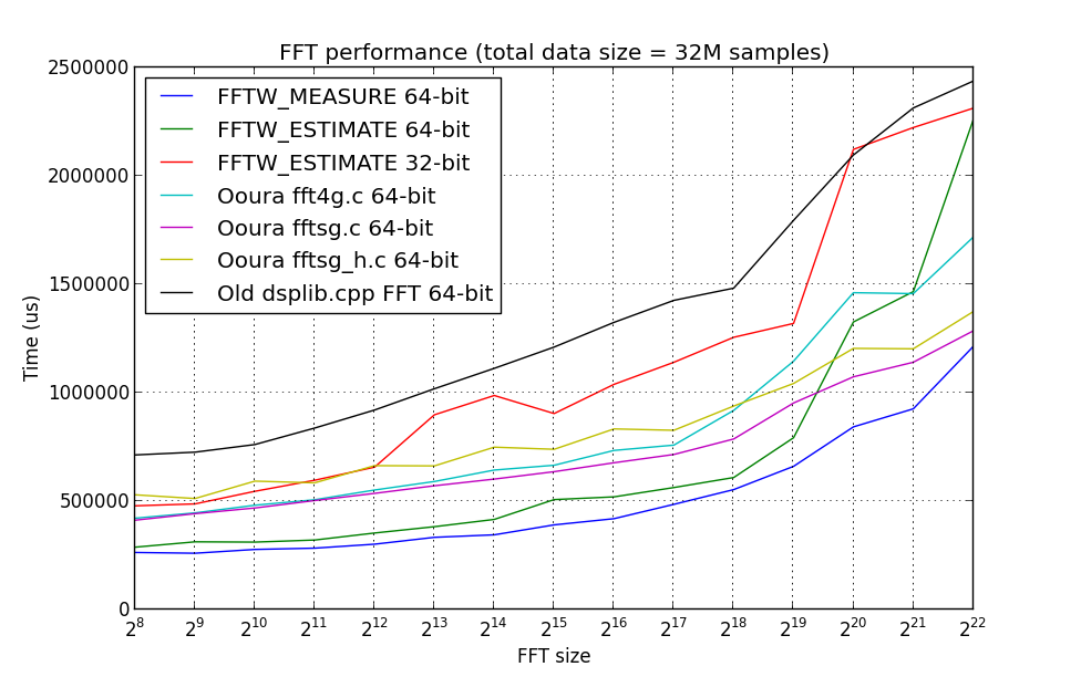
resample.exe - high quality but (depending on the settings used) slow sample rate converter. Some benchmark results can be seen
here. It allows for resampling by any fractional ratio, and delaying the signal by any fractional number of samples. Therefore, it is well suited for pitch correcting and synchronizing recorded test signals, and for audio difference extraction (where accurate synchronization is important). Looping the input sample to generate a periodic waveform is also possible. A number of parameters of the sample rate conversion can be configured:
- interpolation length - controls the quality of the interpolation when the resample ratio or delay is fractional (normally, there is not much point changing the default, unless unusual filter settings are used, or for slghtly faster low quality conversion)
- lowpass filter -6 dB frequency as a fraction of the lower sample rate (by default, it is 0.5)
- lowpass filter impulse response length (longer = faster roll-off, but longer ringing, and somewhat slower processing)
- lowpass filter window type (faster initial roll-off vs. higher stopband attenuation)
- lowpass filter linear vs. minimum phase (the delay is only accurate with the former, and the latter is currently also slightly slower when downsampling by an integer number of octaves)
- quality (1-9): this allows for easy automatic configuration with only the filter frequency (negative for minimum phase filtering) and quality level used as input parameters; the lowpass filter is set up to avoid imaging/aliasing. Use "-q 5 -ff 0.48" to approximate the default "-h" mode of the SoX "rate" effect (or increase the quality to 8 for "-v")
The sample rate adjustment factor, and overall/channel specific gain parameters of the convolve utility are also supported by this program.
sinetest.exe - analyzes the frequency, amplitude, and phase of a sine wave. This is mostly useful with synchronization tones (typically in the kHz range for at least a few seconds) at the beginning and/or end of a loopback recording, the program can calculate the pitch correction, skip time, and channel gain parameters that need to be passed to resample.exe for accurate synchronization and level matching.
testgen.exe - more advanced test signal generator. It supports the following signals:
- sine wave with an exponential frequency and amplitude envelope (for measuring frequency response, THD vs. frequency, and THD vs. level)
- MLS
- JTest (jitter test, Fs/4 tone at -3 dBFS + low level (1 LSB) square wave)
- simple square, sawtooth, triangle, and pulse train, with no anti-aliasing, and a cycle time of integer samples
- stereo noise (white, pink, brown, or other colored noise with an user specified dB/octave slope)
It reads the description of tones to be generated from a text file, each of these has a start time, duration, and usually left/right amplitude, in addition to the parameters specific to that particular signal. Any number of tones can also overlap, allowing for the generation of complex multi-tone signals. The supported output formats are 8, 16, 24, and 32-bit PCM with TPDF dither (the dither is automatically disabled for MLS and JTest).
thd_test.exe - analyzes the frequency response and THD in a (preferably long) sine sweep. It supports THD vs. frequency and level, user specified bandwidth and number of harmonics, and several other parameters. Similarly to groupdel.exe, it only outputs impulse responses, the spectrum of which needs to be visualized with a separate program.
All of the above utilities use 64-bit floats internally. With the exception of mls.exe and testgen.exe, these features are common to all:
- command line parameters can be read from a text file (the format is OPTION = VALUE, the option name should not include the leading '-' character; if the value is a string and includes space(s), double quotes can be used around it)
- text format input files (also for testgen.exe) can use any line endings (LF/CR-LF/CR), and support comments beginning with # or ;
- audio input files can be in any format supported by libsndfile
- audio output files are in WAV format, using 8, 16, 24, or 32-bit PCM, or 32 or 64-bit float samples (floats are not clipped)
- smaller than 32-bit integer PCM format samples are dithered (using a "colored" TPDF dither that moves some of the noise energy into the high frequency range - note that testgen.exe uses white noise instead)
- by default, the pseudo-random number generator used for dithering is seeded from the current time, so the output file is always slightly different; however, the seed can also be specified by the user for repeatable results, or dithering can be disabled if necessary